Matplotlib: Básico
Contents
Matplotlib: Básico#
Tomado de Python de cero a experto by Luis M. de la Cruz Salas is licensed under Attribution-NonCommercial-NoDerivatives 4.0 International
Objetivo general
Practicar el uso de las herramientas de Matplotlib para generar gráficos.
Objetivos particulares
Realizar gráficas de funciones 1D.
Realizar gráficas de funciones 2D.
Realizar gráficas de funciones 3D.
Contenido#
Introducción#
Matplotlib es una biblioteca de basada Python multiplataforma para generar gráficos (plots) en dos dimensiones con las siguientes características:
Se puede usar en una variedad de ámbitos:
Scripts de Python, Shells de IPython, Notebooks de Jupyter, Aplicaciones para Web e Interfaces Gráficas de Usuario (GUI).
Se puede usar para desarrollar aplicaciones profesionales.
Puede generar varios tipos de formatos de figuras y videos:
png, jpg, svg, pdf, mp4, …
Tiene un soporte limitado para realizar figuras en 3D.
Puede combinarse con otras bibliotecas y aplicaciones para extender su funcionalidad.
Arquitectura de tres capas:
Scripting: API para crear gráficas.
Provee de una interfaz simple para crear gráficas.
Está orientada a usuarios sin mucha experiencia en la programación.
Es lo que se conoce como el API de pyplot.
Artist: Hace el trabajo interno de creación de los elementos de la gráfica.
Los Artist (artesanos?) dibujan los elementos de la gráfica.
Cada elemento que se ve en la gráfica es un Artist.
Provee de un API orientado a objetos muy flexible.
Está orientado a programadores expertos para crear aplicaciones complejas.
Backend: El lugar donde se despliega la gráfica. Las gráficas se envían a un dispositivo de salida. Puede ser cualquier interfaz que soporta Matplotlib:
User interface backends (interactive backends): pygtk, wxpython, tkinter, qt4, macosx, …
Hard-copy backends (non-interactive backends): .png, .svg, .pdf, .ps

Figuras y ejes#
import numpy as np
import matplotlib.pyplot as plt
# Creamos un objeto de tipo figure
fig = plt.figure()
<Figure size 640x480 with 0 Axes>
# Creamos unos ejes
ax = plt.axes()
# Definir un tamaño para la figura
fig = plt.figure(figsize=(6.0, 4.0))
ax = plt.axes()
Función plot()#
Grafica un arreglo de coordenadas en 2D usando líneas y/o marcadores.
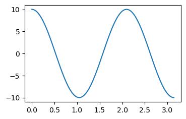
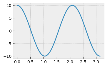
Ejercicio 1 - Gráfica de \(f(x) = \cos(x)\).#
Realice la gráfica de la función \(f(x) = \cos(x)\) usando plt.plot(). Para ello copie el siguiente código en la celda siguiente y ejecútelo.
# Datos
L = ...
A = ...
ω = ...

# Arreglos de coordenadas
x = np.linspace(0, L, 100)
y = A * np.cos(ω * x)

# Graficación
fig = plt.figure(figsize=(4.0, 2.5))
plt.plot(x, y)
plt.show()
Usted debe elegir un valor para:
El estilo (diferente al
default):estilo = ' ... 'Longitud en el eje \(x\) :
L = ...Amplitud de la oscilación \(A\):
A = ...Frecuenta de oscilación \(\omega\):
ω = ...
# Datos

# Arreglos de coordenadas

# Graficación

### BEGIN SOLUTION
# Datos
L = 3.141592
A = 10.0
ω = 3

# Arreglos de coordenadas
x = np.linspace(0, L, 100)
y = A * np.cos(ω * x)

# Graficación
fig = plt.figure(figsize=(4.0, 2.5))
plt.plot(x, y)
plt.show()
### END SOLUTION
Decoración de la gráfica#
Colores
Matplotlib ofrece diferentes colores. Una lista de ellos aquí. Ejemplos de uso de colores aquí
Tipos de líneas
Matplotlib ofrece diferentes tipos de líneas. Una lista de ellos aquí. Ejemplos de uso de colores aquí
Marcadores
Matplotlib ofrece diferentes tipos de marcadores. Una lista de ellos aquí. Ejemplos de uso de colores aquí
Texto en las gráficas
Se puede agregar texto usando la función text(). Mas información aquí. Un ejemplo se puede ver aquí.
Anotaciones sobre las gráficas
Se puede hacer referencia a ciertos puntos sobre la gráfica con anotate(). Mas información aquí. Un ejemplo se puede ver aquí.
Leyendas
Cuando se tienen varias gráficas se puede identificar cada una con una leyenda. Más información aquí. Ejemplos de uso de leyendas aquí.
Estilos
Matplotlib ofrece varios estilos de gráficos. Una lista de ellos aquí. Veamos un ejemplo:
# Obtener la lista de estilos
plt.style.available # 'default'
['Solarize_Light2',
 '_classic_test_patch',
 '_mpl-gallery',
 '_mpl-gallery-nogrid',
 'bmh',
 'classic',
 'dark_background',
 'fast',
 'fivethirtyeight',
 'ggplot',
 'grayscale',
 'seaborn',
 'seaborn-bright',
 'seaborn-colorblind',
 'seaborn-dark',
 'seaborn-dark-palette',
 'seaborn-darkgrid',
 'seaborn-deep',
 'seaborn-muted',
 'seaborn-notebook',
 'seaborn-paper',
 'seaborn-pastel',
 'seaborn-poster',
 'seaborn-talk',
 'seaborn-ticks',
 'seaborn-white',
 'seaborn-whitegrid',
 'tableau-colorblind10']
with plt.style.context('bmh'):
    # Datos
    L = 3.141592
    A = 10.0
    ω = 3

    # Arreglos de coordenadas
    x = np.linspace(0, L, 100)
    y = A * np.cos(ω * x)

    # Graficación
    fig = plt.figure(figsize=(4.0, 2.5))
    plt.plot(x, y)
    plt.show()

# plt.style.use('default')
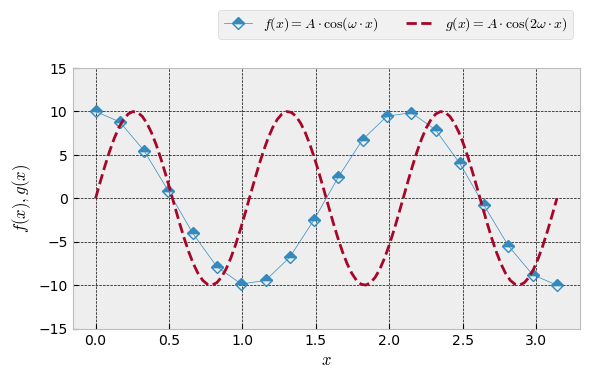
Ejercicio 2 - Replicar una figura#
Intente replicar la siguiente figura:

### BEGIN SOLUTION
# Datos
L = 3.141592
A = 10.0
ω = 3

# Arreglos de coordenadas
x1 = np.linspace(0, L, 20)
x2 = np.linspace(0, L, 100)
f = A * np.cos(ω * x1)
g = A * np.sin(2 * ω * x2)

# Graficación
with plt.style.context('bmh'):
    fig = plt.figure(figsize=(6.0, 4.0))
    plt.plot(x1, f, '-D', lw=0.5, fillstyle='top', label='$f(x) = A \cdot \cos(\omega \cdot x)$')
    plt.plot(x2, g, '--', lw=2.0, label='$g(x) = A \cdot \cos(2 \omega \cdot x)$')
    plt.xlabel('$x$')
    plt.ylabel('$f(x), g(x)$')
    plt.ylim(-15,15)
    plt.legend(loc='best', bbox_to_anchor=(0.5, 0.75, 0.5, 0.5), ncol=2)
    plt.grid(lw=0.5, ls='--', c='k')
    plt.tight_layout()
    plt.savefig('sin_cos.png', dpi=300)
    plt.show()
### END SOLUTION
# Datos

# Arreglos de coordenadas

# Graficación
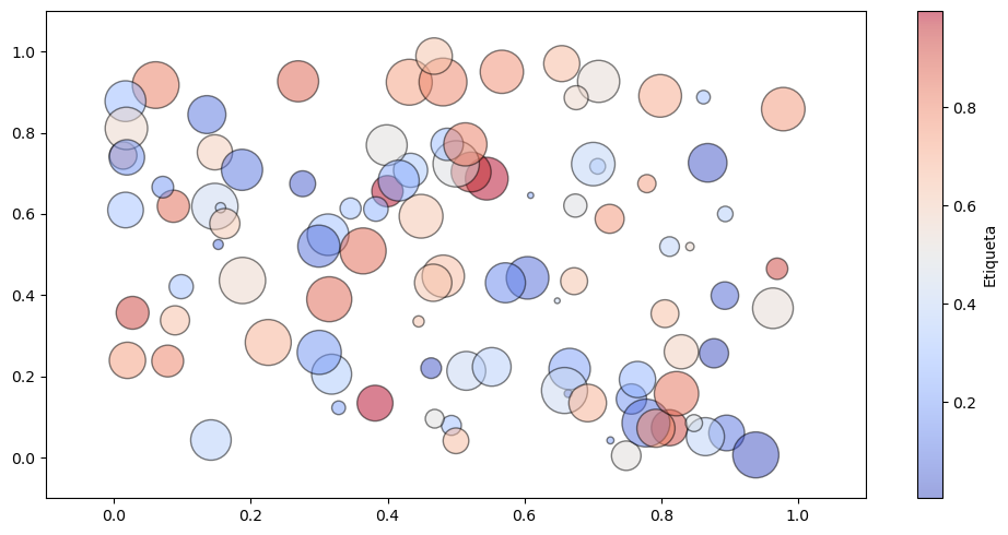
Función scatter()#
Esta función es similar a plot() pero solo grafica marcadores. Veamos el siguiente ejemplo.
fig = plt.figure(figsize=(10,5))
N = 100
xr = np.random.rand(N)  # Coordenada x
yr = np.random.rand(N)  # Coordenada y
c = np.random.rand(N)   # Colores
s = 1000 * np.random.rand(N) # Tamaño de marcador

# Graficación de los puntos
plt.scatter(xr, yr,
            c=c,       # Colores
            s = s,     # Tamaño del marcador
            ec='k',    # Color del borde
            alpha=0.5, # Transparencia
            cmap='coolwarm') # Mapa de color

# Intente agrega el parámetro: marker='$\clubsuit$' en la función anterior

# Barra de colores
plt.colorbar(label='Etiqueta')
plt.xlim(-0.1,1.1)
plt.ylim(-0.1,1.1)
plt.tight_layout()
plt.savefig('imagen1.pdf')
# Graficación de información de un archivo de datos

i_data = np.loadtxt('utils/data/iris_data.txt')

plt.scatter(i_data[:,0], i_data[:,1], alpha=0.75,
            s=100*i_data[:,2], c=i_data[:,3], ec='k', cmap='viridis')
plt.colorbar()
plt.show()
---------------------------------------------------------------------------
OSError                                   Traceback (most recent call last)
~\AppData\Local\Temp\ipykernel_8512\378270237.py in <module>
      1 # Graficación de información de un archivo de datos
      2
----> 3 i_data = np.loadtxt('utils/data/iris_data.txt')
      4
      5 plt.scatter(i_data[:,0], i_data[:,1], alpha=0.75,

~\.conda\envs\OldLibroEnv\lib\site-packages\numpy\lib\npyio.py in loadtxt(fname, dtype, comments, delimiter, converters, skiprows, usecols, unpack, ndmin, encoding, max_rows, like)
   1065             fname = os_fspath(fname)
   1066         if _is_string_like(fname):
-> 1067             fh = np.lib._datasource.open(fname, 'rt', encoding=encoding)
   1068             fencoding = getattr(fh, 'encoding', 'latin1')
   1069             fh = iter(fh)

~\.conda\envs\OldLibroEnv\lib\site-packages\numpy\lib\_datasource.py in open(path, mode, destpath, encoding, newline)
    191
    192     ds = DataSource(destpath)
--> 193     return ds.open(path, mode, encoding=encoding, newline=newline)
    194
    195

~\.conda\envs\OldLibroEnv\lib\site-packages\numpy\lib\_datasource.py in open(self, path, mode, encoding, newline)
    531                                       encoding=encoding, newline=newline)
    532         else:
--> 533             raise IOError("%s not found." % path)
    534
    535

OSError: utils/data/iris_data.txt not found.
puntos = np.loadtxt('utils/data/Projection.txt')
target = np.loadtxt('utils/data/Target.txt')

plt.scatter(puntos[:, 0], puntos[:, 1], lw=0.1,
            c=target, ec='k', alpha=0.5, cmap='viridis')
plt.colorbar(ticks=range(6), label='digit value')
plt.clim(-0.5, 5.5)
---------------------------------------------------------------------------
OSError                                   Traceback (most recent call last)
~\AppData\Local\Temp\ipykernel_6460\505625772.py in <module>
----> 1 puntos = np.loadtxt('utils/data/Projection.txt')
      2 target = np.loadtxt('utils/data/Target.txt')
      3
      4 plt.scatter(puntos[:, 0], puntos[:, 1], lw=0.1,
      5             c=target, ec='k', alpha=0.5, cmap='viridis')

~\anaconda3\envs\LibroEnv\lib\site-packages\numpy\lib\npyio.py in loadtxt(fname, dtype, comments, delimiter, converters, skiprows, usecols, unpack, ndmin, encoding, max_rows, like)
   1065             fname = os_fspath(fname)
   1066         if _is_string_like(fname):
-> 1067             fh = np.lib._datasource.open(fname, 'rt', encoding=encoding)
   1068             fencoding = getattr(fh, 'encoding', 'latin1')
   1069             fh = iter(fh)

~\anaconda3\envs\LibroEnv\lib\site-packages\numpy\lib\_datasource.py in open(path, mode, destpath, encoding, newline)
    191
    192     ds = DataSource(destpath)
--> 193     return ds.open(path, mode, encoding=encoding, newline=newline)
    194
    195

~\anaconda3\envs\LibroEnv\lib\site-packages\numpy\lib\_datasource.py in open(self, path, mode, encoding, newline)
    531                                       encoding=encoding, newline=newline)
    532         else:
--> 533             raise IOError("%s not found." % path)
    534
    535

OSError: utils/data/Projection.txt not found.
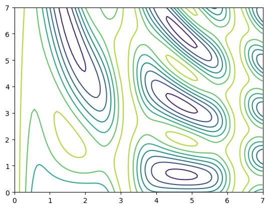
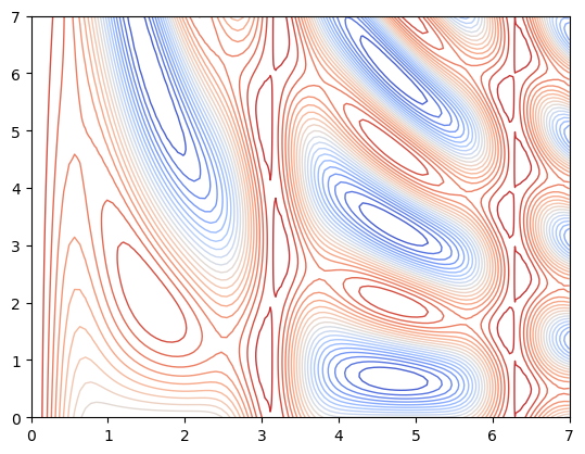
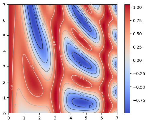
Funciones contour() y contourf()#
Estas funciones permiten graficar datos 3D, (x, y, z) proyectados en contornos en 2D.
f = lambda x, y: np.cos(x) ** 10 + np.sin(y * x / 2) * np.sin(x)
x = np.linspace(0, 7, 100)
y = np.linspace(0, 7, 100)
xg, yg = np.meshgrid(x, y)
zg = f(xg, yg)
plt.contour(xg, yg, zg)
<matplotlib.contour.QuadContourSet at 0x21242842d08>
plt.contour(xg, yg, zg, cmap='coolwarm', linewidths=1.0, linestyles='-', levels=20)
<matplotlib.contour.QuadContourSet at 0x212428a2088>
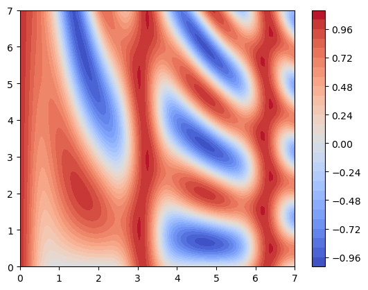
plt.contourf(xg, yg, zg, cmap='coolwarm', levels=30)
plt.colorbar()
<matplotlib.colorbar.Colorbar at 0x212429671c8>
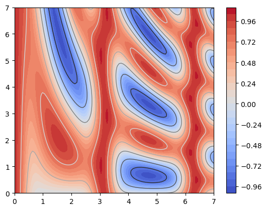
plt.contourf(xg, yg, zg, cmap='coolwarm', levels=30)
plt.colorbar()
plt.contour(xg, yg, zg, cmap='gray', linewidths=1.0, linestyles='-', levels=5)
<matplotlib.contour.QuadContourSet at 0x21243bb6948>
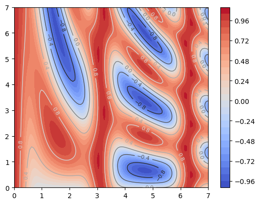
plt.contourf(xg, yg, zg, cmap='coolwarm', levels=30)
plt.colorbar()
contornos = plt.contour(xg, yg, zg, cmap='gray', linewidths=1.0, linestyles='-', levels=5)
plt.clabel(contornos, inline=True, fontsize=8)
plt.savefig('contornos1.pdf')
plt.imshow(zg, extent=[0, 7, 0, 7], origin='lower', cmap='coolwarm')
plt.colorbar()
contornos = plt.contour(xg, yg, zg, cmap='gray', linewidths=1.0, linestyles='-', levels=5)
plt.clabel(contornos, inline=True, fontsize=8)
plt.savefig('contornos2.pdf')
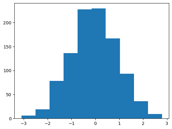
Histogramas hist()#
Esta función permite realizar histogramas simples.
datos = np.random.randn(1000)
plt.hist(datos)
(array([  6.,  19.,  78., 136., 227., 229., 167.,  93.,  36.,   9.]),
 array([-3.09342677, -2.50501462, -1.91660247, -1.32819032, -0.73977818,
        -0.15136603,  0.43704612,  1.02545827,  1.61387042,  2.20228257,
         2.79069471]),
 <BarContainer object of 10 artists>)
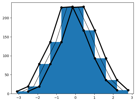
y, x, a = plt.hist(datos)
plt.plot(x[:-1], y, 'ko-', lw=3.0)
plt.plot(x[1:] , y, 'ko-', lw=3.0)
xm = (x[:-1] + x[1:]) * 0.5
plt.plot(xm , y, 'k-', lw=1.0)
print(x)
print(y)
print(xm)
[-3.09342677 -2.50501462 -1.91660247 -1.32819032 -0.73977818 -0.15136603
  0.43704612  1.02545827  1.61387042  2.20228257  2.79069471]
[  6.  19.  78. 136. 227. 229. 167.  93.  36.   9.]
[-2.7992207  -2.21080855 -1.6223964  -1.03398425 -0.4455721   0.14284005
  0.7312522   1.31966434  1.90807649  2.49648864]
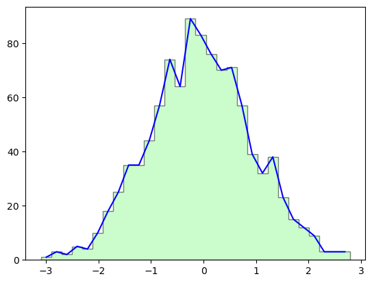
y, x, a = plt.hist(datos, bins=30, alpha=0.5, histtype='stepfilled',
         color='palegreen', edgecolor='k')
plt.plot((x[:-1] + x[1:]) * 0.5 , y, 'b-', lw=1.5)
[<matplotlib.lines.Line2D at 0x212442c0c48>]
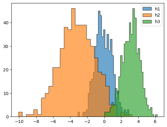
h1 = np.random.randn(500)
h2 = np.random.normal(-3, 2, 500)
h3 = np.random.normal(3, 1, 500)
argumentos = dict(bins=30, alpha=0.65, histtype='stepfilled', edgecolor='k')

plt.hist(h1, **argumentos, label='h1')
plt.hist(h2, **argumentos, label='h2')
plt.hist(h3, **argumentos, label='h3')
plt.legend()
<matplotlib.legend.Legend at 0x21244330608>
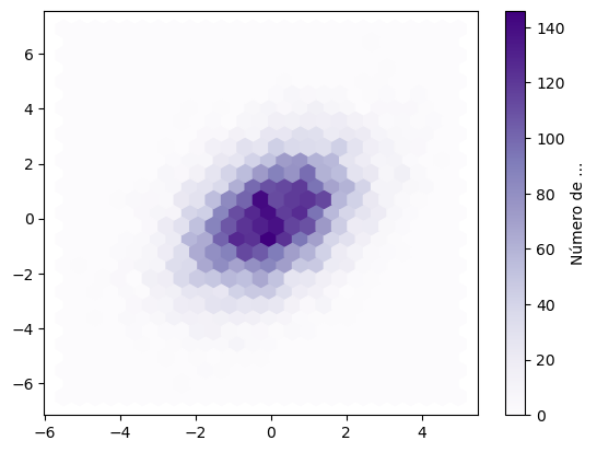
Histogramas bidimensionales hist2d()#
mean = [0, 0]
cov = [[2, 1], [1, 3]]
np.random.multivariate_normal(mean, cov, 10000)
array([[-1.15085703,  0.81664024],
       [-0.21021107,  2.06738182],
       [ 0.07801237, -0.64474262],
       ...,
       [ 1.84465821,  3.31620008],
       [-1.35002631, -3.84774389],
       [-0.17711264, -1.73810014]])
mean = [0, 0]
cov = [[2, 1], [1, 3]]
x, y = np.random.multivariate_normal(mean, cov, 10000).T

plt.hist2d(x, y, bins=25, cmap='Purples')
plt.colorbar(label='Número de ...')
<matplotlib.colorbar.Colorbar at 0x21245b19588>

plt.hexbin(x, y, gridsize=25, cmap='Purples')
plt.colorbar(label='Número de ...')
<matplotlib.colorbar.Colorbar at 0x21245bbcd48>
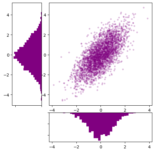
mean = [0, 0]
cov = [[1, 1], [1, 2]]
x, y = np.random.multivariate_normal(mean, cov, 3000).T

fig = plt.figure(figsize=(6, 6))
grid = plt.GridSpec(4, 4, hspace=0.25, wspace=0.25)
ax_m = fig.add_subplot(grid[:-1, 1:])
ax_hy = fig.add_subplot(grid[:-1, 0], xticklabels=[], sharey=ax_m)
ax_hx = fig.add_subplot(grid[-1, 1:], yticklabels=[], sharex=ax_m)

ax_m.plot(x, y, 'o', markersize=3, alpha=0.2, color='Purple')

ax_hx.hist(x, 40, orientation='vertical', color='Purple')
ax_hx.invert_yaxis()

d = ax_hy.hist(y, 40, orientation='horizontal', color='Purple')
ax_hy.invert_xaxis()
Gráficos 3D#
Los siguientes ejemplos muestran cómo realizar gráficos en 3D.
fig = plt.figure()
ax = plt.axes(projection='3d')
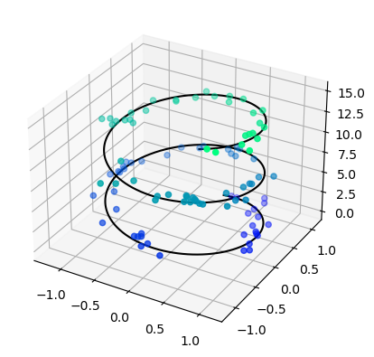
Líneas y puntos en 3D
ax = plt.axes(projection='3d')

# Línea en 3D
zline = np.linspace(0, 15, 1000)
xline = np.sin(zline)
yline = np.cos(zline)
ax.plot3D(xline, yline, zline, 'k')

# Puntos en 3D
zdata = 15 * np.random.random(100)
xdata = np.sin(zdata) + 0.1 * np.random.randn(100)
ydata = np.cos(zdata) + 0.1 * np.random.randn(100)
ax.scatter3D(xdata, ydata, zdata, c=zdata, cmap='winter');
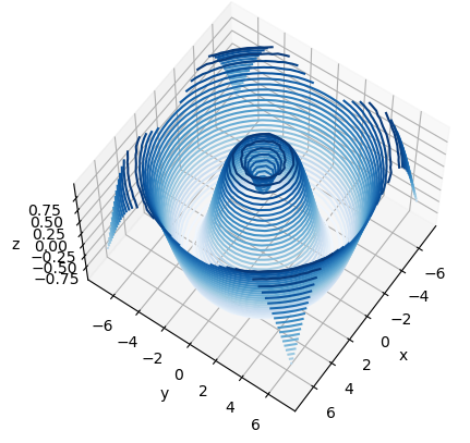
Contornos en 3D
def f(x, y):
    return np.sin(np.sqrt(x ** 2 + y ** 2))
x = np.linspace(-7, 7, 30)
y = np.linspace(-7, 7, 30)

X, Y = np.meshgrid(x, y)
Z = f(X, Y)

fig = plt.figure()
ax = plt.axes(projection='3d')
ax.contour3D(X, Y, Z, 30, cmap='Blues')
ax.set_xlabel('x')
ax.set_ylabel('y')
ax.set_zlabel('z');
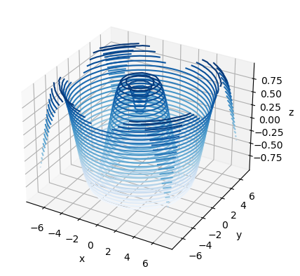
ax.view_init(60, 35)
fig
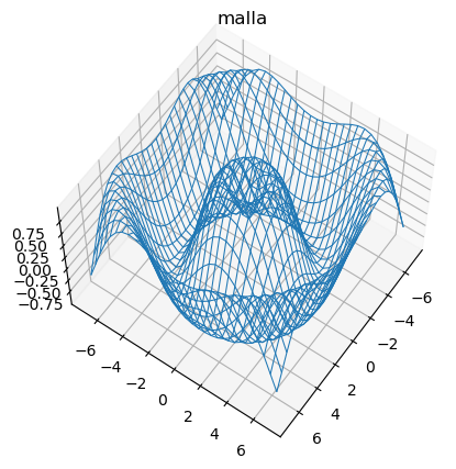
wireframe()
fig = plt.figure()
ax = plt.axes(projection='3d')
ax.plot_wireframe(X, Y, Z, cmap='Blues', linewidth=0.75)
ax.set_title('malla')
ax.view_init(60, 35)
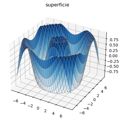
plot_surface()
# Interactividad en 3D
#%matplotlib inline
#%matplotlib notebook
#%matplotlib inline
ax = plt.axes(projection='3d')
ax.plot_surface(X, Y, Z, rstride=1, cstride=1, cmap='Blues',
                edgecolor='gray', linewidth=0.5)
ax.set_title('superficie')
Text(0.5, 0.92, 'superficie')
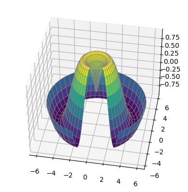
r = np.linspace(0, 6, 20)
theta = np.linspace(-0.9 * np.pi, 0.8 * np.pi, 40)
r, theta = np.meshgrid(r, theta)

X = r * np.sin(theta)
Y = r * np.cos(theta)
Z = f(X, Y)

ax = plt.axes(projection='3d')
ax.plot_surface(X, Y, Z, rstride=1, cstride=1,
                cmap='viridis', edgecolor='gray', linewidth=0.5)
ax.view_init(40, -80)
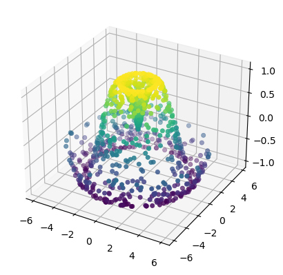
theta = 2 * np.pi * np.random.rand(1000)
r = 6 * np.random.rand(1000)
x = r * np.sin(theta)
y = r * np.cos(theta)
z = f(x, y)

ax = plt.axes(projection='3d')
ax.scatter(x, y, z, c=z, cmap='viridis', linewidth=0.5)
<mpl_toolkits.mplot3d.art3d.Path3DCollection at 0x212460b3b48>
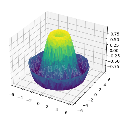
plot_trisurf()
ax = plt.axes(projection='3d')
ax.plot_trisurf(x, y, z,
                cmap='viridis', edgecolor='none');