Numpy (Álgebra Lineal)
Contents
Numpy (Álgebra Lineal)#
Autor: Luis Miguel de la Cruz Salas
Python de cero a experto by Luis M. de la Cruz Salas is licensed under Attribution-NonCommercial-NoDerivatives 4.0 International
Objetivo general
Conocer uno de los módulos (LinAlg) más importantes de la biblioteca Numpy.
Objetivos particulares
Describir una lista de objetivos/actividades que se realizarán en esta práctica.
Hacer énfasis en los métodos y conceptos que se aprenderán y en algunas cuestiones computacionales.
No vaya más allá de tres objetivos particulares y sea muy concreto.
Contenido#
Universal Functions (ufunc)#
Una función universal (ufunc) es aquella que opera sobre arreglos de numpy (´ndarrays´) elemento por elemento, soportando broadcasting y casting, entre otras características estándares.
Se dice que una ufunc es un envoltorio (wrapper) vectorizado para una función que toma un número fijo de entradas específicas y produce un número de salidas específicas.
En Numpy, las funciones universales son objetos de la clase ´numpy.ufunc´.
Muchas de estas funciones están implementadas y compiladas en lenguaje C.
Las ufunc básicas operan sobre escalares, pero existe también un tipo generalizado para el cual los elementos básicos son subarreglos (vectores, matrices, etc.) y se realiza un broadcasting sobre las otras dimensiones.
Broadcasting#
La siguiente figura muestra varios tipos de broadcasting que se aplican en los arreglos y funciones de Numpy.

Observación: Los cuadros en gris tenue son usados para mostrar el concepto de broadcasting, pero no se reserva memoria para ellos.
import numpy as np
import matplotlib.pyplot as plt
x = np.arange(3)
x
array([0, 1, 2])
y = x + 5
y
array([5, 6, 7])
matriz = np.ones((3,3))
matriz
array([[1., 1., 1.],
       [1., 1., 1.],
       [1., 1., 1.]])
vector = np.arange(3)
vector
array([0, 1, 2])
matriz + vector
array([[1., 2., 3.],
       [1., 2., 3.],
       [1., 2., 3.]])
columna = np.arange(3).reshape(3,1)
columna
array([[0],
       [1],
       [2]])
renglon = np.arange(3)
renglon
array([0, 1, 2])
columna + renglon
array([[0, 1, 2],
       [1, 2, 3],
       [2, 3, 4]])
columna * renglon
array([[0, 0, 0],
       [0, 1, 2],
       [0, 2, 4]])
Reglas del broadcasting
Para determinar la interacción entre dos arreglos, en Numpy se siguen las siguientes reglas:
Regla 1. Si dos arreglos difieren en sus dimensiones, el shape del que tiene menos dimensiones es completado con unos sobre su lado izquierdo
Regla 2. Si el shape de los dos arreglos no coincide en alguna dimensión, el arreglo con el shape igual a 1 se completa para que coincida con el shape del otro arreglo.
Regla 3. Si el shape de los dos arreglos no coincide en alguna dimensión, pero ninguna de las dos es igual a 1 entonces se tendrá un error del estilo:
ValueError: operands could not be broadcast together with shapes (4,3) (4,)
Ejemplo 1.#
Mat = np.ones((3,2))
b = np.arange(2)
print(Mat.shape)
print(Mat)
print(b.shape)
print(b)
(3, 2)
[[1. 1.]
 [1. 1.]
 [1. 1.]]
(2,)
[0 1]
Cuando se vaya a realizar una operación con estos dos arreglos, por la Regla 1 lo que Numpy hará internamente es:
Mat.shape <--- (3,2)
b.shape   <--- (1,2)
Luego, por la Regla 2 se completa la dimensión del shape del arreglo b que sea igual 1:
Mat.shape <--- (3,2)
b.shape   <--- (3,2)
De esta manera es posible realizar operaciones entre ambos arreglos:
Mat + b
array([[1., 2.],
       [1., 2.],
       [1., 2.]])
Mat * b
array([[0., 1.],
       [0., 1.],
       [0., 1.]])
Ejemplo 2.#
Mat = np.ones((3,1))
b = np.arange(4)
print(Mat.shape)
print(Mat)
print(b.shape)
print(b)
(3, 1)
[[1.]
 [1.]
 [1.]]
(4,)
[0 1 2 3]
Por la Regla 1 lo que Numpy hará internamente es:
Mat.shape <--- (3,1)
b.shape   <--- (1,4)
Por la Regla 2 se completan las dimensiones de los arreglos que sean igual 1:
Mat.shape <--- (3,4)
b.shape   <--- (3,4)
De esta manera es posible realizar operaciones entre ambos arreglos:
Mat + b
array([[1., 2., 3., 4.],
       [1., 2., 3., 4.],
       [1., 2., 3., 4.]])
Ejemplo 3.#
Mat = np.ones((4,3))
b = np.arange(4)
print(Mat.shape)
print(Mat)
print(b.shape)
print(b)
(4, 3)
[[1. 1. 1.]
 [1. 1. 1.]
 [1. 1. 1.]
 [1. 1. 1.]]
(4,)
[0 1 2 3]
Por la Regla 1 lo que Numpy hará internamente es:
Mat.shape <--- (4,3)
b.shape   <--- (1,4)
Por la Regla 2 se completan las dimensiones de los arreglos que sean igual 1:
Mat.shape <--- (4,3)
b.shape   <--- (4,4)
Observe que en este caso los shapes de los arreglos no coinciden, por lo que no será posible operar con ellos juntos.
Mat + b
---------------------------------------------------------------------------
ValueError                                Traceback (most recent call last)
~\AppData\Local\Temp\ipykernel_13308\4129548612.py in <module>
----> 1 Mat + b

ValueError: operands could not be broadcast together with shapes (4,3) (4,)
Mat.shape = (3,4)
Mat
array([[1., 1., 1., 1.],
       [1., 1., 1., 1.],
       [1., 1., 1., 1.]])
Mat + b
array([[1., 2., 3., 4.],
       [1., 2., 3., 4.],
       [1., 2., 3., 4.]])
Mat + b[np.newaxis,:].T
---------------------------------------------------------------------------
ValueError                                Traceback (most recent call last)
~\AppData\Local\Temp\ipykernel_14428\385980300.py in <module>
----> 1 Mat + b[np.newaxis,:].T

ValueError: operands could not be broadcast together with shapes (3,4) (4,1)
Ufunc disponibles en Numpy#
Para una lista completa de todas las funciones universales disponibles en Numpy refierase al siguiente sitio: https://numpy.org/doc/stable/reference/ufuncs.html#available-ufuncs .
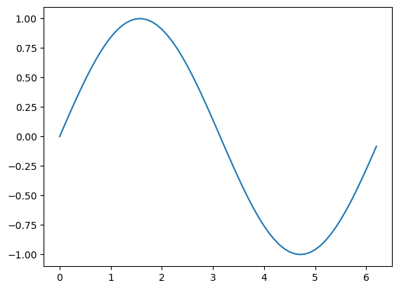
Ejemplo 4.#
x = np.arange(0, 2*np.pi, 0.1)
y = np.sin(x)
plt.plot(x,y)
[<matplotlib.lines.Line2D at 0x279068a7288>]
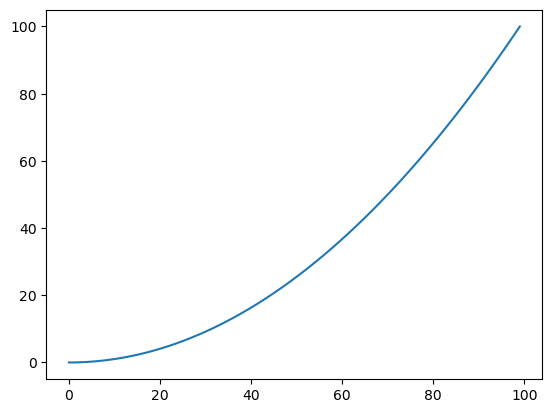
Ejemplo 5.#
x = np.linspace(0, 10, 100)                # Vector renglón
y = np.linspace(0, 10, 100)#[:, np.newaxis] # Vector columna
z = x * y
print(f' x.shape = {x.shape} \n y.shape = {y.shape} \n z.shape = {z.shape}')
 x.shape = (100,)
 y.shape = (100,)
 z.shape = (100,)
z
array([0.00000000e+00, 1.02030405e-02, 4.08121620e-02, 9.18273646e-02,
       1.63248648e-01, 2.55076013e-01, 3.67309458e-01, 4.99948985e-01,
       6.52994592e-01, 8.26446281e-01, 1.02030405e+00, 1.23456790e+00,
       1.46923783e+00, 1.72431385e+00, 1.99979594e+00, 2.29568411e+00,
       2.61197837e+00, 2.94867871e+00, 3.30578512e+00, 3.68329762e+00,
       4.08121620e+00, 4.49954086e+00, 4.93827160e+00, 5.39740843e+00,
       5.87695133e+00, 6.37690032e+00, 6.89725538e+00, 7.43801653e+00,
       7.99918376e+00, 8.58075707e+00, 9.18273646e+00, 9.80512193e+00,
       1.04479135e+01, 1.11111111e+01, 1.17947148e+01, 1.24987246e+01,
       1.32231405e+01, 1.39679625e+01, 1.47331905e+01, 1.55188246e+01,
       1.63248648e+01, 1.71513111e+01, 1.79981635e+01, 1.88654219e+01,
       1.97530864e+01, 2.06611570e+01, 2.15896337e+01, 2.25385165e+01,
       2.35078053e+01, 2.44975003e+01, 2.55076013e+01, 2.65381084e+01,
       2.75890215e+01, 2.86603408e+01, 2.97520661e+01, 3.08641975e+01,
       3.19967350e+01, 3.31496786e+01, 3.43230283e+01, 3.55167840e+01,
       3.67309458e+01, 3.79655137e+01, 3.92204877e+01, 4.04958678e+01,
       4.17916539e+01, 4.31078461e+01, 4.44444444e+01, 4.58014488e+01,
       4.71788593e+01, 4.85766758e+01, 4.99948985e+01, 5.14335272e+01,
       5.28925620e+01, 5.43720029e+01, 5.58718498e+01, 5.73921028e+01,
       5.89327620e+01, 6.04938272e+01, 6.20752984e+01, 6.36771758e+01,
       6.52994592e+01, 6.69421488e+01, 6.86052444e+01, 7.02887460e+01,
       7.19926538e+01, 7.37169677e+01, 7.54616876e+01, 7.72268136e+01,
       7.90123457e+01, 8.08182838e+01, 8.26446281e+01, 8.44913784e+01,
       8.63585348e+01, 8.82460973e+01, 9.01540659e+01, 9.20824406e+01,
       9.40312213e+01, 9.60004081e+01, 9.79900010e+01, 1.00000000e+02])
plt.plot(z)
[<matplotlib.lines.Line2D at 0x27906916208>]
i = plt.imshow(z)
plt.colorbar(i)
---------------------------------------------------------------------------
TypeError                                 Traceback (most recent call last)
~\AppData\Local\Temp\ipykernel_14428\3495214084.py in <module>
----> 1 i = plt.imshow(z)
      2 plt.colorbar(i)

~\anaconda3\envs\LibroEnv\lib\site-packages\matplotlib\_api\deprecation.py in wrapper(*args, **kwargs)
    457                 "parameter will become keyword-only %(removal)s.",
    458                 name=name, obj_type=f"parameter of {func.__name__}()")
--> 459         return func(*args, **kwargs)
    460
    461     # Don't modify *func*'s signature, as boilerplate.py needs it.

~\anaconda3\envs\LibroEnv\lib\site-packages\matplotlib\pyplot.py in imshow(X, cmap, norm, aspect, interpolation, alpha, vmin, vmax, origin, extent, interpolation_stage, filternorm, filterrad, resample, url, data, **kwargs)
   2657         filternorm=filternorm, filterrad=filterrad, resample=resample,
   2658         url=url, **({"data": data} if data is not None else {}),
-> 2659         **kwargs)
   2660     sci(__ret)
   2661     return __ret

~\anaconda3\envs\LibroEnv\lib\site-packages\matplotlib\_api\deprecation.py in wrapper(*args, **kwargs)
    457                 "parameter will become keyword-only %(removal)s.",
    458                 name=name, obj_type=f"parameter of {func.__name__}()")
--> 459         return func(*args, **kwargs)
    460
    461     # Don't modify *func*'s signature, as boilerplate.py needs it.

~\anaconda3\envs\LibroEnv\lib\site-packages\matplotlib\__init__.py in inner(ax, data, *args, **kwargs)
   1410     def inner(ax, *args, data=None, **kwargs):
   1411         if data is None:
-> 1412             return func(ax, *map(sanitize_sequence, args), **kwargs)
   1413
   1414         bound = new_sig.bind(ax, *args, **kwargs)

~\anaconda3\envs\LibroEnv\lib\site-packages\matplotlib\axes\_axes.py in imshow(self, X, cmap, norm, aspect, interpolation, alpha, vmin, vmax, origin, extent, interpolation_stage, filternorm, filterrad, resample, url, **kwargs)
   5479                               **kwargs)
   5480
-> 5481         im.set_data(X)
   5482         im.set_alpha(alpha)
   5483         if im.get_clip_path() is None:

~\anaconda3\envs\LibroEnv\lib\site-packages\matplotlib\image.py in set_data(self, A)
    714                 or self._A.ndim == 3 and self._A.shape[-1] in [3, 4]):
    715             raise TypeError("Invalid shape {} for image data"
--> 716                             .format(self._A.shape))
    717
    718         if self._A.ndim == 3:

TypeError: Invalid shape (100,) for image data
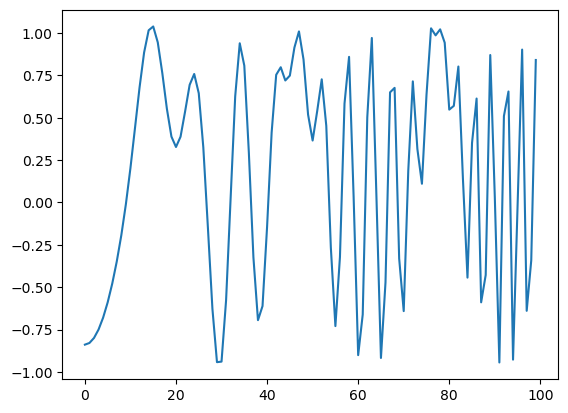
z = np.sin(x) ** 10 + np.cos(10 + y * x) * np.cos(x)
print(f' x.shape = {x.shape} \n y.shape = {y.shape} \n z.shape = {z.shape}')
plt.plot(z)
#i = plt.imshow(z)
#plt.colorbar(i)
 x.shape = (100,)
 y.shape = (100,)
 z.shape = (100,)
[<matplotlib.lines.Line2D at 0x27906ba3088>]
Álgebra lineal#
A = np.linspace(1,9,9).reshape(3,3)
B = np.linspace(1,9,9).reshape(3,3)
a = np.linspace(1,3,3)
b = np.linspace(1,3,3)
print(A)
print(B)
print(a)
print(b)
[[1. 2. 3.]
 [4. 5. 6.]
 [7. 8. 9.]]
[[1. 2. 3.]
 [4. 5. 6.]
 [7. 8. 9.]]
[1. 2. 3.]
[1. 2. 3.]
A.T # Transpuesta de la matriz
array([[1., 4., 7.],
       [2., 5., 8.],
       [3., 6., 9.]])
a * b # Producto de dos vectores elemento por elemento
array([1., 4., 9.])
A * B # Producto de dos matrices elemento por elemento
array([[ 1.,  4.,  9.],
       [16., 25., 36.],
       [49., 64., 81.]])
np.dot(a,b) # Producto punto de dos vectores
14.0
a @ b # Producto punto de dos vectores
14.0
np.dot(A,b) # Producto matriz - vector
array([14., 32., 50.])
A @ b # Producto matriz - vector
array([14., 32., 50.])
np.dot(A,B) # Producto matriz - matriz
array([[ 30.,  36.,  42.],
       [ 66.,  81.,  96.],
       [102., 126., 150.]])
A @ B # Producto matriz - matriz
array([[ 30.,  36.,  42.],
       [ 66.,  81.,  96.],
       [102., 126., 150.]])
c = b[:,np.newaxis] # Agregamos una dimension al vector (vector columna)
print(c.shape)
print(c)
(3, 1)
[[1.]
 [2.]
 [3.]]
c * a # Producto externo: vector columna por vector renglón
array([[1., 2., 3.],
       [2., 4., 6.],
       [3., 6., 9.]])
Paquete linalg#
Esta biblioteca ofrece varios algorimos para aplicarlos sobre arreglos de numpy (véa aquí la referencia). Todas operaciones de álgebra lineal de Numpy se basan en las bibliotecas BLAS (Basic Linear Algebra Suprograms ) y LAPACK (Linear Algebra Package ) para proveer de implementaciones eficientes de bajo nivel de los algoritmos estándares.
Estas biblioteca pueden proveer de versiones altamente optimizadas para aprovechar el hardware óptimamente (multihilos y multiprocesador). En estos casos se hace uso de bibliotecas tales como OpenBLAS, MKL ™, y/o ATLAS.
np.show_config() # Para conocer la configuración del Numpy que tengo instalado
blas_mkl_info:
    libraries = ['mkl_rt']
    library_dirs = ['C:/Users/RYZEN/anaconda3/envs/LibroEnv\\Library\\lib']
    define_macros = [('SCIPY_MKL_H', None), ('HAVE_CBLAS', None)]
    include_dirs = ['C:/Users/RYZEN/anaconda3/envs/LibroEnv\\Library\\include']
blas_opt_info:
    libraries = ['mkl_rt']
    library_dirs = ['C:/Users/RYZEN/anaconda3/envs/LibroEnv\\Library\\lib']
    define_macros = [('SCIPY_MKL_H', None), ('HAVE_CBLAS', None)]
    include_dirs = ['C:/Users/RYZEN/anaconda3/envs/LibroEnv\\Library\\include']
lapack_mkl_info:
    libraries = ['mkl_rt']
    library_dirs = ['C:/Users/RYZEN/anaconda3/envs/LibroEnv\\Library\\lib']
    define_macros = [('SCIPY_MKL_H', None), ('HAVE_CBLAS', None)]
    include_dirs = ['C:/Users/RYZEN/anaconda3/envs/LibroEnv\\Library\\include']
lapack_opt_info:
    libraries = ['mkl_rt']
    library_dirs = ['C:/Users/RYZEN/anaconda3/envs/LibroEnv\\Library\\lib']
    define_macros = [('SCIPY_MKL_H', None), ('HAVE_CBLAS', None)]
    include_dirs = ['C:/Users/RYZEN/anaconda3/envs/LibroEnv\\Library\\include']
Supported SIMD extensions in this NumPy install:
    baseline = SSE,SSE2,SSE3
    found = SSSE3,SSE41,POPCNT,SSE42,AVX,F16C,FMA3,AVX2
    not found = AVX512F,AVX512CD,AVX512_SKX,AVX512_CLX,AVX512_CNL
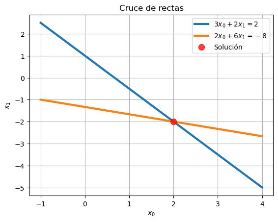
Ejemplo 6.#
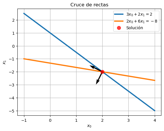
Cruce de dos rectas:
\( \begin{array}{ccc} 3x_0 + 2x_1 & = &2 \\ 2x_0 + 6x_1 & = &-8 \end{array} \)
En forma de sistema lineal:
\( \left[ \begin{array}{cc} 3 & 2 \\ 2 & 6 \end{array} \right] \) \( \left[ \begin{array}{c} x_{0} \\ x_{1} \end{array} \right] = \) \( \left[ \begin{array}{c} 2 \\ -8 \end{array} \right] \)
Podemos calcular el cruce de las rectas resolviendo el sistema lineal:
A = np.array([[3, 2],[2,6]] )
b = np.array([2,-8])
print("Matriz A : \n",A)
print("Vector b : \n", b)
sol = np.linalg.solve(A,b) # Función del módulo linalg para resolver el sistema
print("Solución del sistema: ", sol)
Matriz A :
 [[3 2]
 [2 6]]
Vector b :
 [ 2 -8]
Solución del sistema:  [ 2. -2.]
Graficamos las rectas y la solución:
Las ecuaciones de las rectas se pueden escribir como:
\( \begin{array}{ccc} \dfrac{3}{2}x_0 + x_1 & = & \dfrac{2}{2} \\ \dfrac{2}{6}x_0 + x_1 & = & -\dfrac{8}{6} \end{array} \Longrightarrow \begin{array}{ccc} y_0 = m_0 x + b_0 \\ y_1 = m_1 x + b_1 \end{array} \text{ donde } \begin{array}{ccc} m_0 = -\dfrac{3}{2} & b_0 = 1 \\ m_1 = -\dfrac{2}{6} & b_1 = -\dfrac{8}{6} \end{array} \)
def graficaRectas(x, y0, y1, sol):
    plt.plot(x,y0,lw=3,label = '$3x_0+2x_1=2$')
    plt.plot(x,y1,lw=3,label = '$2x_0+6x_1=-8$')
    plt.scatter(sol[0], sol[1], c='red', s = 75, alpha=0.75, zorder=5, label='Solución')
    plt.xlabel('$x_0$')
    plt.ylabel('$x_1$')
    plt.title('Cruce de rectas')
    plt.grid()
    plt.legend()
m0 = -3/2
b0 = 1
m1 = -2/6
b1 = -8/6
x = np.linspace(-1,4,10)
y0 = m0 * x + b0
y1 = m1 * x + b1

graficaRectas(x, y0, y1, sol)
eigen = np.linalg.eig(A)
eigen
(array([2., 7.]),
 array([[-0.89442719, -0.4472136 ],
        [ 0.4472136 , -0.89442719]]))
def dibujaEigen(eigen, sol):
    xv,yv = np.meshgrid([sol[0], sol[0]],[sol[1], sol[1]])
    u = np.hstack( (eigen[1][0], np.array([0, 0])) )
    v = np.hstack( (eigen[1][1], np.array([0, 0])) )
    vec = plt.quiver(xv,yv,u,v,scale=10, zorder=5)
dibujaEigen(eigen, sol)
graficaRectas(x, y0, y1, sol)

Forma cuadrática#
\( f(x) = \dfrac{1}{2} \mathbf{x}^T A \mathbf{x} - \mathbf{x}^T \mathbf{b} + c \)
\( A = \left[ \begin{array}{cc} 3 & 2 \\ 2 & 6 \end{array} \right], x = \left[ \begin{array}{c} x_{0} \\ x_{1} \end{array} \right], b = \left[ \begin{array}{c} 2\\ -8 \end{array} \right], c = \left[ \begin{array}{c} 0\\ 0 \end{array} \right], \)
\( f^\prime(x) = \dfrac{1}{2} A^T \mathbf{x} + \dfrac{1}{2} A \mathbf{x} - \mathbf{b} \)
Cuando \(A\) es simétrica: \( f^\prime(x) = A \mathbf{x} - \mathbf{b} \)
Entonces un punto crítico de \(f(x)\) se obtiene cuando \( f^\prime(x) = A \mathbf{x} - \mathbf{b} = 0\), es decir cuando \(A \mathbf{x} = \mathbf{b}\)
from mpl_toolkits.mplot3d import Axes3D

def dibujaSurf(A,b):
    def f(A,b,x,c):
        return 0.5 * (x.T * A * x) - b.T * x + c

    size_grid = 30
    x1 = np.linspace(-3,6,size_grid)
    y1 = np.linspace(-6,3,size_grid)

    xg,yg = np.meshgrid(x1,y1)
    z = np.zeros((size_grid, size_grid))

    for i in range(size_grid):
        for j in range(size_grid):
            x = np.matrix([[xg[i,j]],[yg[i,j]]])
            z[i,j] = f(A,b,x,0)

    fig = plt.figure()
    #surf = fig.gca(projection='3d')
    surf.plot_surface(xg,yg,z,rstride=1,cstride=1, alpha=1.0, cmap='viridis')
    surf.view_init(15, 130)
    surf.set_xlabel('$x_0$')
    surf.set_ylabel('$x_1$')
    surf.set_zlabel('$f$')
    return xg, yg, z
xg,yg,z = dibujaSurf(A,b)
---------------------------------------------------------------------------
NameError                                 Traceback (most recent call last)
~\AppData\Local\Temp\ipykernel_14428\1148520655.py in <module>
----> 1 xg,yg,z = dibujaSurf(A,b)

~\AppData\Local\Temp\ipykernel_14428\2526263686.py in dibujaSurf(A, b)
     19     fig = plt.figure()
     20     #surf = fig.gca(projection='3d')
---> 21     surf.plot_surface(xg,yg,z,rstride=1,cstride=1, alpha=1.0, cmap='viridis')
     22     surf.view_init(15, 130)
     23     surf.set_xlabel('$x_0$')

NameError: name 'surf' is not defined
<Figure size 640x480 with 0 Axes>
dibujaEigen(eigen, sol)
graficaRectas(x, y0, y1, sol)
cont = plt.contour(xg,yg,z,30,cmap='binary')
---------------------------------------------------------------------------
NameError                                 Traceback (most recent call last)
~\AppData\Local\Temp\ipykernel_14428\4098156203.py in <module>
      1 dibujaEigen(eigen, sol)
      2 graficaRectas(x, y0, y1, sol)
----> 3 cont = plt.contour(xg,yg,z,30,cmap='binary')

NameError: name 'xg' is not defined

Algoritmo del descenso del gradiente
\(
\begin{array}{l}
\text{Input} : \mathbf{x}_0, tol \\
\mathbf{r}_0 = \mathbf{b}-A\mathbf{x}_0 \\
k = 0 \\
\text{WHILE}(\mathbf{r}_k > tol) \\
\qquad \mathbf{r}_k \leftarrow \mathbf{b}-A\mathbf{x}_k \\
\qquad \alpha_k \leftarrow \dfrac{\mathbf{r}_k^T\mathbf{r}_k}{\mathbf{r}_k^T A \mathbf{r}_k} \\
\qquad \mathbf{x}_{k+1} \leftarrow \mathbf{x}_k + \alpha_k \mathbf{r}_k \\
\qquad k \leftarrow k + 1 \\
\text{ENDWHILE}
\end{array}
\)
def steepest(A,b,x,tol,kmax):
    steps = [[x[0,0], x[1,0]]]
    r = b - A @ x
    res = np.linalg.norm(r)
    k = 0
    while(res > tol and k < kmax):
        alpha = r.T @ r / (r.T @ A @ r)
        x = x + r * alpha
        steps.append([x[0,0],x[1,0]])
        r = b - A @ x
        res = np.linalg.norm(r)
        k += 1
        print(k, res)
    return x, steps
xini = np.array([-2.0,-2.0])
tol = 0.001
kmax = 20

xs, pasos = steepest(A,b[:,np.newaxis],xini[:,np.newaxis],tol,kmax)
1 5.384289904692891
2 3.5895266031285917
3 1.3400899318346766
4 0.8933932878897847
5 0.3335334941455197
6 0.22235566276367916
7 0.08301278076510733
8 0.055341853843404884
9 0.0206609587682041
10 0.013773972512135697
11 0.00514228307119734
12 0.0034281887141298767
13 0.001279857119940566
14 0.00085323807996087
def dibujaPasos(xi, sol, pasos):
    pasos = np.matrix(pasos)
    plt.plot(pasos[:,0],pasos[:,1],'-')
    plt.scatter(xi[0], xi[1], c='yellow', s = 75, alpha=0.75, zorder=5, label='Solución')
    plt.scatter(sol[0], sol[1], c='red', s = 75, alpha=0.75, zorder=5, label='Solución')
dibujaEigen(eigen, sol)
graficaRectas(x, y0, y1, sol)
cont = plt.contour(xg,yg,z,30,cmap='binary')
dibujaPasos(xini, sol, pasos)
---------------------------------------------------------------------------
NameError                                 Traceback (most recent call last)
~\AppData\Local\Temp\ipykernel_14428\2273471878.py in <module>
      1 dibujaEigen(eigen, sol)
      2 graficaRectas(x, y0, y1, sol)
----> 3 cont = plt.contour(xg,yg,z,30,cmap='binary')
      4 dibujaPasos(xini, sol, pasos)

NameError: name 'xg' is not defined